I initially found it quite difficult to comprehend how aggregation works via the mongo documentation. To understand this concept, I went through a bit of trial and error and eventually came up with a successful solution. So here’s what I learned.

Within mongodb, the aggregation framework provides two ways to aggregate data. The standard aggregation pipeline and and the map reduce paradigm.

According to the documentation, the aggregation pipeline provides better performance and a more coherent interface. However, if you require much more complex aggregations and your dataset is larger than 16 megabytes, map-reduce is needed.

In my case, the time series data has two or three records per second collected over several months – so my data set significantly exceeded the 16 megabyte limit.

First thing, your TIME field must be mongo’s Date type to use the aggregation pipeline.

Aggregation Pipeline

The aggregation pipeline, in my opinion, is a little more simpler to understand than map-reduce.

There are two phases, the match or projection phase followed by a group phase. The nice thing about the aggregation framework is that we can use some pre-defined operators.

We start off with the $project operator. With $project we can reshape the document stream by renaming, adding, or removing fields.

Price and Volume are set as 1, as to include them in the projection. Next I create a year, month, day, and hour field using the date operators provided. What this projection is essentially doing is reshaping each entry to effectively cut off anything less than an hour.

So if we had two entries like:
Tue Mar 18 2014 19:01:20
Tue Mar 18 2014 19:50:20

We are essentially removing the minute and second property, so the time can be represented as:
$year = 2014
$month = 03
$day = 18
$hour = 19

So now that the data is projected, we can begin the group phase to group duplicate entries like the two above together. The $group operation must have an _id which will be what we are grouping together. Also, we can use some more aggregation operators to compute our additional fields. In the above group operation, I am grouping by year, month, day and hour. I am taking the price field and calculating the average of all the grouped entries with $avg, as well as calculating the total volume with $sum. The result is an aggregated time series. The above aggregation won’t work for my dataset, for one my dataset is too large and I would like fifteen minute intervals instead of one hour or one minute.

Map-reduce

Map-reduce is similar to $project and $group. The first operation is the map, which is similar to $project. Inside my defined map function, we call emit which emits a key-value pair that the reduce function accepts as parameters.In the above example I get the time in minutes, determine which ‘quarter hour’ the time falls in and create the projection key time_at_minute.

Using a similar example.

Tue Mar 18 2014 19:01:20
Tue Mar 18 2014 19:10:20
Tue Mar 18 2014 19:50:20

The first two entries would be grouped into:
Tue Mar 18 2014 19:00 (FIRST QUARTER)

and the final entry into:
Tue Mar 18 2014 19:45 (FOURTH QUARTER)

The reduce function takes the emit from the map and returns a result object. The key, in my example, is the time. The values parameter is a list of any values (defined in map) that correspond to the key (or projection).

In this example I manually perform some calculations because we don’t have access to the fancy operators. At the end, I return an object with whatever data I hope to get out of the aggregation.

Finally, we can include a query. This query will be run against the initial collection. In this example I want to aggregate all records occurring after a specified time.

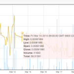
Now with your aggregated data, you can plot some fancy graphs, replace your current dataset to reduce it’s enormous side, or whatever else you feel like doing.